Questions and Answers on Principal Component Analysis.

Errata

At 11:58 in the youtube video lecture, the eigengenes are the columns in the u matrix. However in the slides before, I would make up that eigengenes are the rows in transposed v. What am I seeing incorrectly here?

Nice catch. I am just missspeaking. As a correlary you can see in the code that I am taking values from Vt.

What is PCA

Is PCA considered as a kind of linear regression which shows the correlation between two variables?

No, not really. However, the principal component will show that the variance of some variables are better described as a linear combination of the variables. That is would be a sign of co-variation of the variables.
It seems as though, in the stackexchange answer, they want to convey that the first principal component is the eigenvector with the highest eigenvalue when factoring out covariance. What is the importance of factoring out covariance, and would there not be biological significance in the covariance?

All data analysis aims at explaining the variation in the data. PCA is a nice way to do so for covarying data. The point is that you factor out the covariation to specifically study the covariation.
- Could you clarify in which situation of unsupervised learning it is useful to use PCA rather than k-means clustering? Could we combine k-means clustering and PCA in the same analysis as comfirmation?
- How do we select between Clustering and PCA as unsupervised learning techniques?
  
  PCA focuses more directly on the explanation of the underlying phenomena driving the variation of the data. If there is one or a few factors with a linear influence to many of the observed variables, then PCA is a great method to find such factors. It is a very good idea to perform both types of analysis side by side to see if you get corroborating results.

Applications of PCA

- What is the main use of PCA in life science? Is it to more easily visualize data (through dimensionality reduction) or to determine the most important features/variables in terms of variance?
- Could we say that PCA is a clustering algorithm? Can it be used for clustering except visualization, feature selection and dimensionanily reduction?
  
  No PCA is not a clustering technique. The analysis itself does not give you any groups of data points. PCA have multiple applications. It can be used for visualization, for dimensionality reduction and as a technique to give mechanistic explanation of any linear effects that you are trying to assess. It can also be used for determining biases of your patient material, for missing value imputations. A very nice and applied explanation: One example is in genomics, where, when we set up an experiment, we have biological and technical replicates. Usually what we are looking for is a biological difference between two conditions, and to be sure that this is the case PCA can be used as a kind of quality control. What we want to observe is that most of the variance is explained by biology and not by technical factors, i.e. that principal component 1 is larger than principal component 2. I hope that this was clear enough and a correct explanation. If not, looking at the PCA of this article might help: Here the authors RNA-sequenced for differential gene expression on Zika-virus infected cells using two different sequencing platforms (MiSeq and NextSeq). When they did the PCA, they could show that 50 % of the variance between the samples was due to whether the cells were infected with Zika virus or not, and 20 % the variance was due to the platform that they used (MiSeq or NextSeq).

Variance explained and singular values

What are the singular values themselves, and how can they be interpreted?

They are directly related to the amount of variance explained by each principal component. As explained here, you can directly use them to calculate the proportion of the variance explained for each PC.
Could you explain how the variance is calculated, and how the sum of the variance are correlated to the sum of the total error?

Variance of uncorrelated variables are always additive. So, are the variances explained by the principal components.
When transforming a dataset into PC: is there no net loss of information, as a result of reducing its dimensions?

No, not if all dimensions are used. Otherwise, yes, obviously.
- PCA uses maximum variance as a key driving element for the dimension reduction. Does this mean that the smaller effects are lost or neglected in PCA? Or should one simply look at higher component numbers to find these smaller effects.
- For eg. transcriptional noise of genes expression can be regulated by multiple factors. Of which TF, accessibility, ribosomal availability, small regulatory elements (RNA) etc. TF is one of the biggest regulator and small RNA (microRNA) have smaller role as compared to TF. In this scenario if we are interested to study the effects from microRNA then can we use PCA? Or will the small effect of microRNA be ignored in the PCA? Or will I have to look at PC 10 or PC 20 instead of PC1?
  
  Yes, subtile differences migh be lost in the analysis.

Relation PCA and SVD

Is SVD simply a way of performing PCA.

Yes, SVD is a method for PCA. A more elaborate answer can be found here.
Does SVD allow for faster computation, or are there any other advantages of using one method over the other?

Normally one use SVD as it is more numerically stable than other methods to compute PCA.

Orthogonality of Principal components

A requirement in Principal Component Analysis is that the individual principal components are linearly independent (and therefore orthogonal to each other). Does this requirement only apply in respect to the initial/first principal component? Otherwise I don’t understand how this method would be applicable for more than 3-dimensional plots.

No all Principal components are orthogonal to each other. N-dimensional spaces can contain max N vectors that are orthogonal to each other.

Interpretation of principal components

In the video in the example about the height and the weight it is said that the second principal component seems to be more interesting for interpreting the results but I didn´t manage to understand the reason for that.

You would normally assume that a tall person allso is a heavy person. This implies that there is a linear relationship between squared length and weight. That relationship will be explaining most of the variation of your data, and end up in PC1. The PC1 would normally not be interesting to study, at least not in e.g. T2D studies. However, hopefully, PC2 will capture the BMI, which might be of larger interest.
What is the reason for the transformation from data axes to principal component axes? The transformed graph will always look like a sphere, with all the principal component vectors beeing the same lenght.

Good question. After the transformation the PCs will have an eigen value attached to them so that you know how much of the variance they explain. Particularly PC1 will be the linear combination of data that optimally explains the variation of the data.
The PCA plots given in papers almost always have the axis labelled as Principal component 1 or PC1 and so on, but it never mentions the actual element or the feature based on which this component refers to. Why is it done so? Wouldn’t it be more useful and intuitive to use the name of the feature itself (based on which the component is actually made) as the axis title?

These are linear combinations of features, hence ther is no single feature to refer to.
Also, is there any particular reason for why the genes in the notebook pointing in either positive or negative directions in both PCs are more interesting than those pointing positive on one PC and negative on the other?

In general, features that covary between the PCs can be signs of there being a bias in the patients, that we might be able to detect by studyin the eigen genes.
What is their relationship with the original data (e.g. “eigen gene 1” with “gene 1” values)?

An eigen gene is the linear combination of patients that would explain most of the variation of the data.
Is there any reason why the principal components are pointing in the direction they are pointing? I mean for example in the second picture in VaderPlas reading material, wouldn’t it be the same if the second principal component was pointing up instead of down?

No this is an arbitrar choice. You can fip the signs of the elements in the eigen patients and the eigen genes and they would still explain the same thing.

Eigen genes and Eigen Samples

In the video lecture at around 6:50 , It is said and understood that the columns of U represent the projections of the data onto the PC1. But what does it mean that the rows of Vt represent projection of different samples inside of X?

I like the concepts of Kluwer et al.. Eigen genes is the best representation of how a gene behave, and eigen assays (or eigen experiments, eigen patients) are representations of how patients behave.
Do the concepts of eigen genes and eigen assays/samples only come up when you do a SVD for PCA (as in the jupyter notebook and Kluwer et al. reading)? Or are the same concepts relevant when you do just a PCA (as was done in the VanderPlas reading with the commands: pca = PCA(n_components=2), pca.fit(X))? I do not understand the relationship between PC1 and PC2 and eigen genes and eigen samples/assays.

There are some subtle differenes between PCA and SVD, so they PCs and the eigen vectors differs a by a scalar factor. Modulo those differences: If the data in the introduction to PCA was gene expression values for two different patients, the components in the figure for cell 6 would be the eigen patients one and two and the direction of the axises of the input space is the eigen genes. The eigen gene equivalent is also available through pca.components_ in cell 4.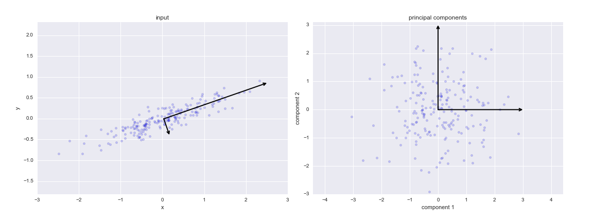
In the JupyterNotebook, I don’t understand why the Eigenpatients (and not the Eigengenes) are used to obtain the genes that are most responsible for the difference between cancer types.

The first eigen patient, is a what a gene expression profile from the single patient that would explain most of the variation in the data would look like.
In the notebook the SVD is used to get eigengenes and eigenpatients, are these the principal components? From what I understood it seems that they explain just the variance of patients and of genes respectively, how would a PCA function choose which of these to use as principal components to explain the variance of the whole dataset?

They PCs are telling you what linear combinations of variables that will explain the most of the variation of the variables.
Could you please explain the last part of the stackexchange answer, from the point that it starts talking about matrices. I don’t understand what are the eigenvectors and eigenvalues.

That part of the answer is not essential for the understanding of PCA, however: A covariance matrix is a description of how much variation you have in the data in each dimension(in the diagonal) as well as how much the datapoints dimensions are covarying with (non-diagonal elements). The answer makes the point that PCA is a projection from input space to a co-ordinate system where there is no covariation in the data, i.e. the covariation matrix is diagonal.

Relation to other techniques

tSNE is another most commonly used clustering technique apart from PCA. I understand that tSNE is probabilistic while PCA is statistical in nature. When is PCA preferred and when is tSNE preferred?

Neither of the techniques are clustering techniques. PCA is a simpler technique than tSNE, and gives mechanistical insights to the data. It’s worth noting as well that many consider tSNE to be overused.
What is the difference between orthogonal and oblique rotation methods to interpret the components?

I guess you mean factor analysis. PCA is a type of factor anaysis.

Number of dimensions of the data

Is it possible or common to have higher dimensionality in PCA, or is it limited to the 3 correlations and PC1/PC2?

The upper bound of the number of the PCs are the rank of the expression matrix, which often equate to the min of number of columns and rows of the analyzed matrix.
How do you determine how far the dimensionality reduction should be taken (i.e. how many principal components to keep)?

It is a matter of a) how much variance remains to be explains and b) your taste.
Are Eigen vectors unit vectors and which direction do they generally point? Also Do eigen values give the significance of a particular component and help to choose the components with highest significance?

Both the eigen genes and eigen assays of Kluwer et al are unitary vectors. There is no significance associated with them, per se.
Is there any threshold to select the number of components? How can we decide the number of components to have a more accurate analysis?

The question directly relates to how much of the variance you want to cover.

Preprocessing

Could you go through this piece of code in your notebook (In [3])?
```
  from numpy.linalg import svd
  X = combined.values
  Xm = np.tile (np.mean(X, axis=1)[np.newaxis].T, (1,X.shape[1]))
  U, S, Vt = svd(X-Xm, full_matrices=True, compute_uv=True)
```
What is actually happening here? I do understand that the generated output is the U matrix containing the eigensamples and genes, S matrix which is the singularvalue matrix and Vt which is the samples and eigengens. However, I do not follow what is happening beforehand and what the Xm is used for.

Great question. We often centralize (i.e. remove the mean of each probe) our data before SVD. In the code, np.mean(X, axis=1)[np.newaxis].T will render a one dimensional matrix with the mean expression value for each gene. Subsequently, you tile, i.e. copy that 1-dimensional vector in X.shape[1] copies into a matrix od the same dimension as X.

Kernelized versions of PCA

Do the parameters you are investigating have to be linearly correlated or can they be non-linear correlated?

Not in the standard formulation of PCA. However, there are kernelized versions of PCA
Can one combine the dimension reduction in PCA with the addition of a dimension in kernel function to linearly separate data points? > Yes you can.

Linear transformations

In the article “SVA analysis of gene expression data” they write that n is the columns of gene expression data, and that if r<n the transcriptional responses of the genes may be captured with fewer variables if we use gi’ instead of gi (gi being the gene transcriptional response). Also they write that due to presence of noise r=n in any real gene expression analysis application. Could you clarify this? I have a hard time understanding what r is, why r has to be less than n for gi’ to capture the response instead of gi, and why r is always equal to n due to noise in real applications?

I am guessing that you are reffering to Kluwer et al. This is hard to explain if you did not read algebra and geometry in your curiculum. r is the rank of the matrix, which in some cases can be lower than the lowest dimension n.
“If r < n, the transcriptional responses of the genes may be captured with fewer variables using g’i rather than gi. This property of the SVD is sometimes referred to as dimensionality reduction” In the above statement, it says that if the rank of the assay matrix X is less than the number of columns, (i.e- assays), the transcriptional response can be defined by fewer variables. How does this happen? Will the reduction in rank of the assay matrix reduce number of dependencies?

r<n only when a column or row in the matrix X is a linear combination of the other.

Notebook

What do the sentences “the genes pointing in a positive/negative direction for the two components” at the end of the jupyter notebook mean?

The genes with the higest resp lowest Eigen patients 1 and 2.
In the final steps of the exercise presented in the notebook, the aim is to identify the genes that are more likely to be responsible for the observed difference among of lung cancer data points. The eigenpatients associated with the genes are investigated, and the KRT17 gene is identified as the minimal eigengene for eigenpatient 1 (i.e. the gene that least explains the variance in the dataset) and as the maximal eigengene for eigenpatient 2 (i.e. the gene that most explains the variability). Is this correct? If so, does this mean the KRT17 gene explains the variation in the dataset better than the other 2 identified genes? Could you please elaborate a bit further the interpretation of these results?

Your interpretation that KRT17 drives both eigen patient 1 and 2 and hense is a better explanation of the data than the other genes could be right. KRT17 is a known cancer related gene. At this point of the analysis, it is not fully clear what the biological interpretation of PC2 is. From the eigen gene plot, it is however clear that PC1 seem to capture the difference beween LUAD and LUSC.

Other

The whole “Kluwer et al.” paper is beyond my comprehension. From the Jupyter notebook I’ve barely understood what SVD does in general, but I still don’t get the main concepts.

It would be helpful if you point out at what part of the paper you stopped understanding the text.
What’s the form of the eigenvectors?

Vectors?
Are they “ranked” according to their relevance in describing the overall variance?

Yes that is right. PC1 describes more or equal of the variance than PC2.
If you have m patients and n genes, you’ll obtain m+n eigenvectors in total, but the PCA components should be mxn (one per dimension): how can you compare the two things?

No, you have <= min(m,n) principal components.
The VaderPLas page seems to describe PCA in two different ways in the case of low-dimensional data and in the case of high-dimensional data: I’m failing to reconnect this two descriptions. The first case is based on the process of projecting the data points on the component’s line: this is fairly easy to imagine (and to do) for bi- or tri-dimensional data, but is this concept applicable to high-dimensional data as well? I would say that in theory it’s feasible, but then, in the digits example, it is suggested to imagine the construction of a single picture as: image(x) = mean + x_1 (basis1) + x_2(basis2) + x_3*(basis3)+… It appears to me that the concept of “projections” is lost here. I also wonder if it’s possible to apply this latter kind of simplification to bi-dimensional data sets. According to the example, image(x) is a single data point and [X_1, X_2, …] are its pixel values. It is also stated that PCA can calculate both the “mean” and the 64 basis and that you can obtain a close-resembling reconstruction of the digit’s picture only by exploiting the first 8 components. If the “mean” and the various “basis” are constant for every data point, that would mean that only the first 8 pixels values (the upper line of each picture) are enough to characterize 10 different types of digits (hard to believe). On the other hand, if these values are not constant, that would mean that PCA works on clusters and not on the whole data set (which would make perfectly sense, but then why this fact is not even mentioned?).

I excluded this part of the text as preparational material, as it might be confusing, The word [projection}(https://en.wikipedia.org/wiki/Projection_(mathematics)) has the meaning of a function that maps data points in one space to another space. Also, in the eigen digit example, VanderPlas only keep 8 values, but they do so together with their “basis” (eigen digits), which each have the same dimension as the orignial images. However, given that they have a large number of images 8 values per image + 8 eigen digits is a compression of data.

General properties of PCAs

Are the eigenvectors given from the SVD or are they needed beforehand?

They are given by the SVD.
Is there a limit of how many dimensions PCA can be applied to? Does the maximum number of dimensions that PCA is suitable for depend on the size and/or quality of the data set? In that case, how?

The notebook contains an example of PCA on 20k dimensions. There might be that you can hit an over limit by using even more dimensions, however, I have not experienced any problems with the size of the problem.

Difference between PCA and SVD

- According to wikipedia SVD is a different name for PCA, depending on the field of application. But I read somewhere else that PCA is built upon SVD, and it seemed like the PCA method was an extension somehow. So, is there a difference between the two and, in that case, what is it? * Would calculating a covariance matrix between genes in a microarray and then performing a PCA yield exactly the same result as performing SVD on it?
- I don’t really understand, is SVD a method that is always used to perform PCA or are they two different/independent methods for dimensionality reduction but that they combined together? (I felt that SVD was difficult to understand and I don’t think I understood exactly its connection with PCA).
  
  SVD is an algorithm for performing PCA (give and take some small considerations).
  A more elaborated answer:
  “What is the difference between SVD and PCA? SVD gives you the whole nine-yard of diagonalizing a matrix into special matrices that are easy to manipulate and to analyze. It lay down the foundation to untangle data into independent components. PCA skips less significant components. Obviously, we can use SVD to find PCA by truncating the less important basis vectors in the original SVD matrix.”
Can you explain more about the relationship between PCA and SVD?

Yes I can.

Singular Value Decomposition

(4 votes) I found it hard to understand what the three matrices in the SVD represented. Could you explain this a bit more?

Not very much more than i.e. the description in Kluwer et al. Hopefully this will become clear after the seminar.

Eigenvectors and Eigenvalues

(5 votes) In what circumstances are we interested in the properties of “eigenpatients”, rather than “eigengenes”?

The eigenpatient contains the variation within the patients, e.g. the first eigenpatient contains the most descriptive difference between the patients. So the eigenpatient is a vector containing one value per gene that gives the relative weight of that gene. Conversely, the eigengenes contains the variation within the genes, e.g. the first eigengene contains the most descriptive difference between the genes. So the eigengene is a vector containing one value per patient that gives the relative weight of that patient.
(5 votes) I did not understand what we should extract from SVD. I understand we can see the single value matrix as the equivalent of PCA “explained variance”, but what do we do then? Do we take the corresponding eigenassay column or the eigengene row for further analysis? Honestly, I don’t understand what is contained in the other two matrices defined in SVD.

Right, it might be a bit abstract at first. I will try to run some examples during the seminar, if you were not convinced by the examples in the video.
(3 votes) What exactly is S and why is it a diagonal matrix? Why is the Eigengene matrix transposed?

The S matrix is a diagonal matrix containing the eigenvalues. The eigengene matrix is transposed as it is the way it comes out from a SVD.
Do the Eigengenes and Eigensamples with their values actually exist in the data (= are there samples and genes which have exactly those values) or are those hypothetical ‘genes’ and ‘samples’ which describe the variance across the dataset?

No, there is no individual sample or gene that takes the same shape as the eigengene. They are an average behavior across all genes/samples.

Explained variance

In the summary of the PCA section in the book by Jake Van der Plas, the author states that ‘Certainly PCA is not useful for every high-dimensional dataset, but it offers a straightforward and efficient path to gaining insight into high-dimensional data’ In his examples, a plot of the cumulative explained variance resembled a pareto curve (as above). Is this behaviour a requirement for a successful principle component analysis?

It is not a requirement on the problem, instead it is a property of the analysis. 1st PC contains the most of the variance, 2nd PC the next-to most of the variance, etc. As the PCs are ordered, each new component adds a smaller and smaller contribution to the variance explained. Hence, the type of plot you see above.
(3 votes) What information could the S matrix give us in the jupyter notebook example?

The S matrix (also called sigma matrix) in a SVD contains the eigen-values. In this context, they are indicating the relative importance of the PCs of how well they explain the variance within your gene-expression matrix.
Is it possible that for instance when investigating 10 genes/dimensions that at least 4 of them accounts for equally large variance and are thus equally relevant and therefore PCA cannot convert the data into dimensions that are displayable?

That is entirely possible.
(3 votes) What are some good ways to identify an optimal number of reduced dimensions?

The amount of explained variation is a typical mean to identify which components that are relevant.

Covariation

- I don’t really get the covariance matrix. Do we have to compute that to be able to perform PCA?
  
  No.
- Why would we need to look at the covariation of each pair of data points? In the explanations of PCA you just look for the dimensions that explains most of the variance.
  
  Yes that is all a PCA does for you, it finds a rotation where the the variance in the data is best explained in order of the principal components. * Is it that when this is done computationally (and not by eye as in the explanations) the best way to compute this is to base it on calculations of covariance between all data points? No, there is no separate covariance calculations involved. Just let the SVD do its job. In practice the PCA replaces linear combinations of covarying variables with new variables.

Dimensionality Reduction

When doing a dimensionality reduction using PCA it is said that it involves “zeroing out” one or more of the smallest principal components. Are these considered outliers or why is it necessary to “zero out” these? Also, what exactly does it mean to “zero out”?

VanderPlas means that you can make a dimensionality reduction of your problem by just selecting a subset of the principal components.

Number of PC’s to extract.

(2 votes) When PCA is used in machine learning do we need to do dimensional reduction to 3D or 2D or can they handle higher dimensions? And does a higher dimension generally show a clearer picture than a lower dimension?

You frequently strive to reduce your problem to as few components as possible, but not less.
When combining components do you / the computer try different variations to see which one has the best separation, or do we decide ourselves what we think is appropriate?

You have to choose the number of dimensions yourself.
(2 votes) As I understood, to plot the results of a PCA in 2D we need to select two principal components. What can we do if PC1 and PC2 can only explain a small amount of the total variance? Is there a way to include more components within the PCA plot?

You are free to include as many components you want. However, they are sorted in the order of amount of explained variance. Hence if your first two components did not explain that much variance your third component is also not likely to explain much.

Applications

What are the applications of singular value decomposition？

Any situation where you would like to explain the covariation in multi-dimensional data with a fewer number of components.

Regularization

Both PCA and SVD are associated with the regularization term. Can you explain what regularization is and how it is linked with PCA and SVD?

No, I do not think that is right. Neither of the methods are using regularization.
In VaderPlas section on principle component analysis it is briefly explained that PCA’s main weakness is its tendency to be highly affected by outliers in the data. This has neccecitated the development of robust variants which can account for this by itterativly discarding datapoints. Is there a point where this can lead to overfitting the data where eliminating datapoints can compromise the validity of the constructed components? Is this commonplace in PCA?

There is no really nice way to characterizing overfittings to data for unsupervised learning. However, just as for supervised learning, the more parameters you introduce the more prone an algorithm is prone to fit a particular dataset. Conversely, if you select a too rigid model (with too few parameters), it will fail to generalize.
It is said that PCA is affected by outliers and that some variants of the method can compensate for that or remove them in some way, but I have difficulties understanding how outliers can be identified as such and not just as points showing an actual effect, especially when the aim is to investigate the data.

VanderPlas mention SparsePCA and explains that it uses a regularization scheme called L1-penalty, i.e. it penalizes not just for squared errors of the decomposition, but also for number of non-zero elements in each principal components. Feel free to try the method yourself in e.g. the jupyter notebook.

Kluwer et al. nomenclature

(5 votes) To me the eigengenes/eigensamples and principal components seem like kind of the same thing, what’s the difference?

None. Eigengenes/eigensamples is just a more direct nomenclature.
(3 votes) I had problems with understanding what eigenassays are. From what I understood they correspond to the columns (U_k) in the left (m x n) matrix U in X=USV^T and it is mentioned that they are analogous to principal components. I still don’t understand what they represent in a gene expression analysis.

The eigenassay contains the variation within the patients, e.g. the first eigenassay contains the most descriptive difference between the assays. So the eigenassay is a vector containing one value per gene that gives the relative weight of that gene.
Is the “first Eigen gene” means the first principal component and the “second Eigen gene” means the second principal component? So are they both the linear combination of a set of different genes? In Jupyter notebook’s illustration, it seems really similar to how we illustrating PC1, PC2, etc.
Eigen genes. These illustrate the linear combinations of genes that explains the variance of the genes. First one describes the most, the second explains most of the variance when the variance of the first gene-compination is removed. Here we only explore the first two component, but one could plot the other ones as well.)

Yes, the nomenclature in the notebook follows the section 2 of Kluwer et al.
Can you explain the connection between PCA and eigengenes/eigensamples again? Does the eigengenes and/or eigensamples describe the principal components of the data set?

Yes, Kluwer et al. calls principal components eigengenes and eigenassays.

Limitations of PCA

(3 votes)) It is mentioned in “principal component analysis summary” that PCA is less useful for high-dimensional data sets. Is this due to the loss of information or is it other factors limiting the use of PCA?

I dissagree, VanderPlas states that: “Certainly PCA is not useful for every high-dimensional dataset, but it offers a straightforward and efficient path to gaining insight into high-dimensional data.”, that is not really the same thing as you state. PCA is frequently used in high dimensional data, as we are in more need of dimensionality reduction in high dimensional data.
It is mentioned that PCAs main weakness is outliers in your data. Does this mean that there are examples of when PCA or dimensionality reduction is possible but not recommended? Such as when there is a lot of variance between samples and data?

The main limitation is that PCA is a linear technique. If the association between two variable is not linear, you might not catch such associations.
In Kluwer paper, it is demonstrated that the difference between SVD and other analysis methods is the ability to detect the ‘weak signal’. How could we define this ‘weak signal’, if it means that when the data cannot be clustered by k-means/GMM, or the dimension of data is much larger, SVD and PCA could be the better choice?

Weak signals can be sometimes be captured by other clustering methods as well. What is great with PCA is that it allows you to strip of one effect at the time from the data (just as Kluwer et al. demonstrates).

Notebook

In the notebook (PCA of Carcinomas) it is explained that the data from both types of cancer are merged a just one single dataset and from this “new merged data set” the principal components are obtained which are later used for the SVD analysis. I don’t quite understand how you plot the “new merged data set” for obtaining the principal components when you only have the transcripts count as the variable? I mean, in the youtube video you explain that a single data set from patients could be plotted in order to get the principal component 1, though there you had 2 variables (height and weight). In the notebook we only have one single variable (counts of transcripts), so how does the code produce the principal component? Does it choose random transcript counts and plot them against each other?

Each of the two sets contains patients’ gene expression values (about 20k gene exression values per patient). Here the data is given as a 500 x 20k array, patients as columns, genes at rows. You add the patients containing the two types of cancer in one large set,which here is represented as a 1k x 20k matrix. This is a typicalthing that is easier viewed in the notebook directly.

Design of Experiments

(2 votes) In your youtube video you say that the difference we can see in the first plot in the jupyter notebook could be due to biases in the data sets, such as that they have been normalized separately. How can such biases be avoided? Moreover, is the data always normalized before performing PCA and if so how is the normalization done?

You conduct your experiment exactly the same way for all samples. That is easier said than done, though.

Other types of Dimensionality Reduction

(4 votes) Is there any other dimensionality reduction methods utilizing a metric other than the covariance measure? I.e. can you capture other features of the data in question by the same procedure as PCA?

One related type of analysis that is using a different orthogonality criterium than PCA is Independent Component Analysis (ICA).
(2 votes) Other dimensionality reduction methods such as t-SNE are often also used for example in gene expression analysis. When do we prefer to use PCA in front of other methods, and could we then for example also use t-SNE on the data in the jupyter notebook?

t-SNE is a non-linear technique. We wont cover it here, but it is great for visualisation of multidimensional data. Feel free to try it out in the notebook example, it is relatively straightforward to implement.
It has been shown that PCA is not useful for every high-dimensional dataset. Being the outliers affection in the data one of the PCA’s main weakness.
Scikit-Learn is one of the strongest iterative alternatives to discard poorly described data points from the dataset. This method contains interesting variants on PCA, RandomizedPCA and SparsePCA.
RandomizedPCA approximates the first few principal components in a fast but non-deterministic way. While SparsePCA introduces a regularization term enforcing sparsity of the components.
In which cases, would it be better to use RandomizedPCA, achieving a fast discard of the data points and when it would be better to introduce and regularize the components through the SparsePCA variant?

Why don’t you find out by trying them out?

Outliers

When you have outliers in the PCA, how do you know if you can discard them? The text says that you can discard “data points that are poorly described by the initial components”, but what defines if they are poorly described?

You! It is a subjective call.
In the lecture video, the most extreme genes for Eigen Patient 1 and 2 are considered the most relevant. How do we know these are not outliers? Has the data been filtered before the analysis?

No I do not say that they are more relevant, just that they describe the most of the variation in the data. They could contain outlier data, so it might be worth plotting their expression values.